Why Flow Analysis?
Sprint velocity and burndown charts tell you whether you delivered — they don’t tell you how reliably or where work is getting stuck. A team can hit every sprint goal while still having work that sits untouched for two weeks before anyone picks it up.
Flow analysis answers different questions: How long does work actually take? Is delivery time getting better or worse? Where does work slow down or pile up? Which items are at risk right now?
AgileViz connects to your Azure DevOps board and gives you a cycle time visual built directly from your team’s real delivery data. The same principles apply whether you’re looking at a requirement-level backlog (User Stories, PBIs) or a portfolio-level board (Features, Epics) — the patterns, metrics, and analysis techniques in this guide work at any level.
This guide explains what you’re looking at and how to turn it into action.
What You’re Looking At
When you generate the visual, you’ll see a panel for each column on your board — one for In Progress, one for Review, one for UAT, and so on, depending on how your team’s board is set up.
Each panel contains:
- Dots — one for each work item in progress or completed during your selected date range
- A shaded band — marking the range between your p50 and p85 delivery times for that column
- A sparkline below each panel — showing how much work was in that column each day
- A stats row at the bottom — showing delivery time statistics at a glance
Below all the panels, a second stats row shows board-level statistics.

Don’t worry if this feels like a lot at first — each element is explained in the sections below.
Cycle Time: How Long Work Takes


Cycle time is how long a work item spends moving through your board — from when work starts until it is complete. The cycle time shown in AgileViz is board cycle time: from when work first starts on an item to when work completes.
Each blue dot in a column panel represents one completed work item. Its position on the vertical axis (the y-axis) tells you how many days that item spent in that column.
A dot sitting high up took a long time. A dot near the bottom moved through quickly.
Cycle time is measured per item rather than averaged because averages hide important information. An average of 8 days could mean every item took exactly 8 days — or it could mean half took 2 days and half took 14. Those two situations call for very different responses.
Your board configuration matters. AgileViz uses Azure DevOps state categories — Proposed, In Progress, and Completed — to determine where cycle time starts and ends. Each of your board states is assigned to one of these categories, which determines which columns count toward cycle time. If a column that represents active work is mapped to Proposed instead of In Progress, items in that column won’t be counted toward cycle time and your numbers will be understated. If you see cycle time values that seem too low, check your board’s column-to-state mappings in Azure DevOps.
Reading the Scatter Plot


The visual uses a scatter plot — each dot’s horizontal position (x-axis) shows when that item was completed, and its vertical position (y-axis) shows how many days it took.
A few things about the axes are worth knowing:
The x-axis shows column exit date, not entry date. Items on the left completed the column earlier in your date range; items on the right completed more recently. This lets you spot trends — are items taking longer now than they were three months ago?
The y-axis uses a logarithmic scale. This sounds technical but has a practical benefit: it prevents a handful of very long items from squashing all the other dots to the bottom. Both short items (1–3 days) and long items (30+ days) remain readable on the same chart.
Percentiles: A Better Way to Measure


Instead of asking “what is the average cycle time?”, percentiles ask a more useful question: “What percentage of items complete within a given number of days?”
For example, a p50 of 5 days means half of your work items complete within 5 days. A p85 of 12 days means 85% of items complete within 12 days — and 15% take longer.
This matters for setting service level agreements (SLAs) with stakeholders. Rather than promising “things take about a week”, you can say “85% of items are done within 12 days”. That’s a commitment you can measure against — and it’s based on what your team has actually demonstrated.
The p50 line is a good indicator of your typical delivery time. The p85 line is a good basis for an SLA — it’s achievable most of the time, while still being honest about occasional slower items.
The p50–p85 Band


The shaded band in each column panel spans from the p50 line to the p85 line. Its height tells you something important: how predictable your delivery is.
A short band means most items take a similar amount of time. Your team’s pace is consistent and your commitments are reliable.
A tall band means delivery time varies a lot. Some items finish quickly, others take much longer. This makes it harder to give stakeholders a reliable estimate, and it often signals that something in your process is inconsistent — unclear work sizing, dependency issues, or interruptions.
The band gives you a quick visual answer to “can we trust our estimates?” without needing to calculate anything.
The vertical position of the band also tells you something when comparing columns. A band sitting higher up means that column takes longer — items spend more days there than in columns with lower bands. Scanning across your board, the column with the highest band is where work slows down the most.
Variance Color: At a Glance
Each column header in the stats strip is color-coded to signal variance level at a glance. A blue value is consistent; an orange or red value has high variance and deserves a closer look.
The color coding uses the same data as the p50-p85 band height — it’s a summary signal to help you quickly identify which columns need attention when you’re scanning across the board.

WIP: How Much Is in Flight
WIP stands for work in progress — the number of items in a column at any given time.


There’s a well-established relationship in flow theory: more WIP leads to longer cycle times. When too much work is piling into a column, items wait longer before anyone can progress them. Reducing WIP — even when it feels counterintuitive — is one of the most reliable ways to speed up delivery.
The WIP sparkline below each column panel shows how WIP changed day by day during your selected date range. A flat line means a steady pace. A spike means work piled up — look for what happened around that time.
A consistently high WIP in one column is a signal that the column is a bottleneck — work is arriving faster than it can be processed.
Throughput and Little’s Law
Throughput is the number of items your team completes per unit of time — typically measured as items per week reaching the Done column. It’s measured at the board exit point, not at any intermediate step.
Little’s Law is the fundamental relationship that connects the three core flow metrics:
Cycle Time = WIP ÷ Throughput
If your team has 8 items in progress and completes 4 per week, the average cycle time is 2 weeks. This isn’t a management technique — it’s a mathematical law that holds for any stable system.
The AI analysis checks whether your board obeys Little’s Law by comparing the expected cycle time (average WIP ÷ throughput per day) to the actual measured p50 cycle time. When they match (ratio near 1.0), the system is in stable equilibrium — WIP, throughput, and cycle time are consistent with each other.
When they diverge, something is off: items may be entering or leaving the measurement window inconsistently, WIP may be changing rapidly, or the board may not have reached steady state during your selected date range.
The practical takeaway: reducing WIP is the most direct lever for reducing cycle time. Little’s Law guarantees the relationship. If throughput stays constant and you reduce WIP, cycle time drops proportionally.
Lead Time vs. Cycle Time
The board stats strip below the column panels shows two related but different measurements:
Board Cycle Time is the time from when work starts to when it’s done. It measures active delivery time.
Board Lead Time is the time from when work is created (or requested) to when it’s done. It includes any time work spent waiting before it even reached the board.
The Lead Time–Cycle Time gap (labeled LT-CT Gap in the board stats strip and AI report) is the difference between the two. A large gap means work is sitting in a backlog for a long time before your team even picks it up. For stakeholders who submitted a request, that waiting time is invisible — but it’s part of their experience of how long things take.

If your team wants to improve the experience for people waiting on work, the gap is often where the biggest opportunity lies.
In-Progress Items


Not all dots on the chart represent completed work. Hollow dots are items that were still in progress as of your selected end date — they haven’t crossed the finish line yet.
Their horizontal position shows either their exit date for the column or the end date of your range if they are still in that column. Their vertical position shows how long they’ve been in the column so far.
A hollow dot sitting above the p85 line on the right edge of a column is an aging item — it has already been in that column longer than 85% of your completed work. That’s a signal worth acting on.
Spotting Bottlenecks
With all the elements above in mind, you can now read across your board to find where work is slowing down.
Signs that a column is a bottleneck:
- High p85 — items regularly take a long time to move through
- Tall p50-p85 band — delivery time in this column is unpredictable
- High or spiky WIP — more work piles into this column than can be processed
- Aging in-progress dots — items are stuck above the p85 line right now


When you see several of these signals in the same column, that’s where to focus on improvements.
A single high p85 could just mean that column handles complex work. But high p85 plus high WIP plus tall p50-p85 band usually points to a process problem worth investigating.
What a Bottleneck Looks Like
Here’s a UAT column from a real board where all four signals are present at once:
The dots split into two clusters — a fast group near the bottom and a slow group scattered up to 30+ days. This bimodal pattern is a hallmark of an unreliable process: some items sail through, others get stuck. The p50-p85 band is tall and the p85 is red.
Notice the WIP sparkline: it shows a sustained buildup that correlates directly with the slow cluster. A column with inherently variable delivery time is vulnerable — but it’s often an event that triggers the real damage. A team member on vacation, a batch of complex work arriving at once, or an external dependency stalling reviews can cause WIP to spike. That spike traps items longer, amplifying the underlying variability into something much worse. The bimodal scatter and the WIP spike aren’t independent problems — they feed each other.
The effects also ripple outward. When one column backs up, upstream columns can’t drain — their WIP rises too, staggered in time. Look across the sparklines on a board with a bottleneck and you’ll often see echoes of the same spike in adjacent columns. And even after the triggering event ends, the elevated WIP takes time to work through. The spike is past, but items trapped during the buildup are still aging in the column. The effect lingers.
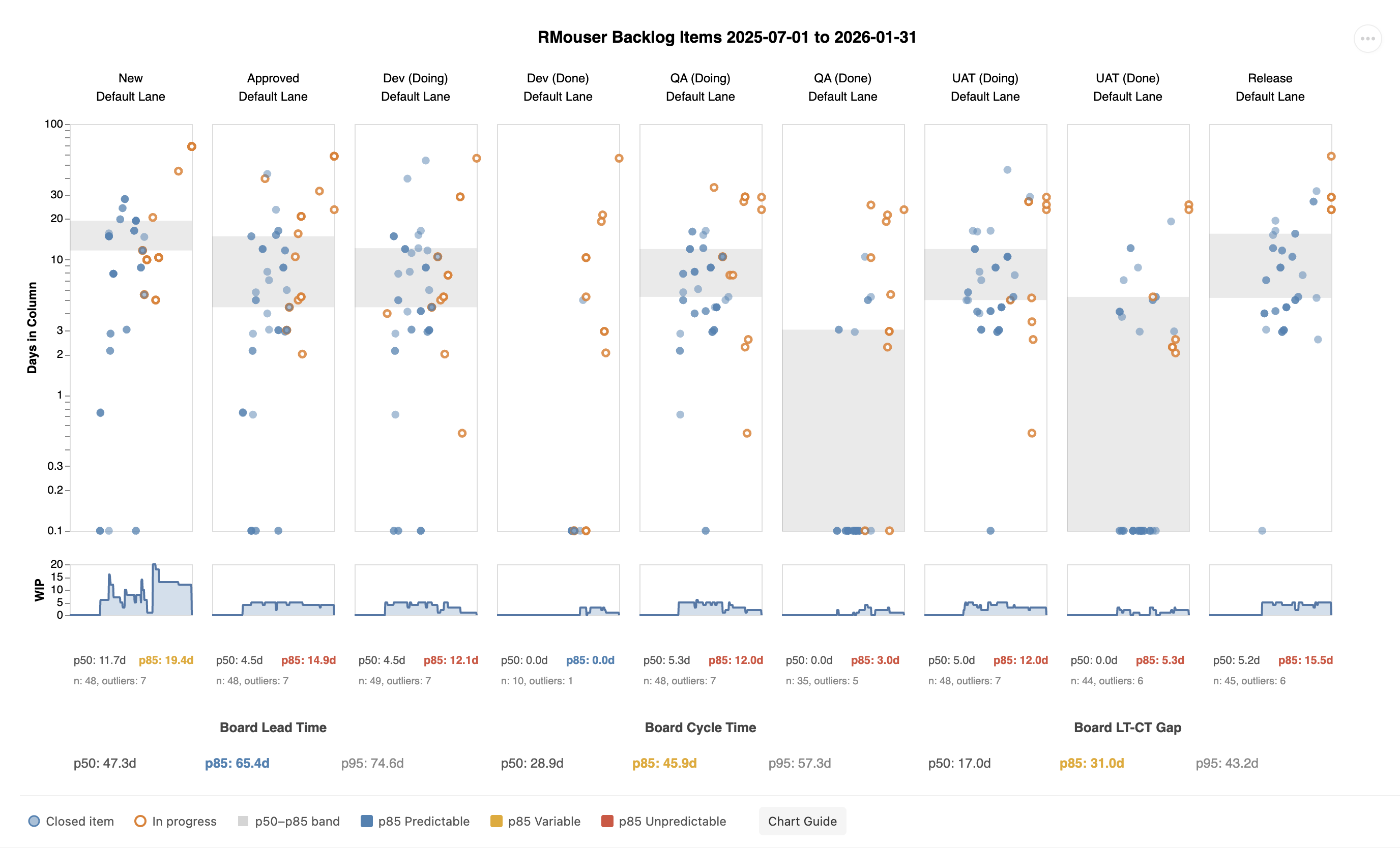
One Bad Column Affects the Entire Board
The impact of a single bottleneck column goes beyond that column. Notice how the UAT column stands out from all the others on the board below — every column is healthy except one:
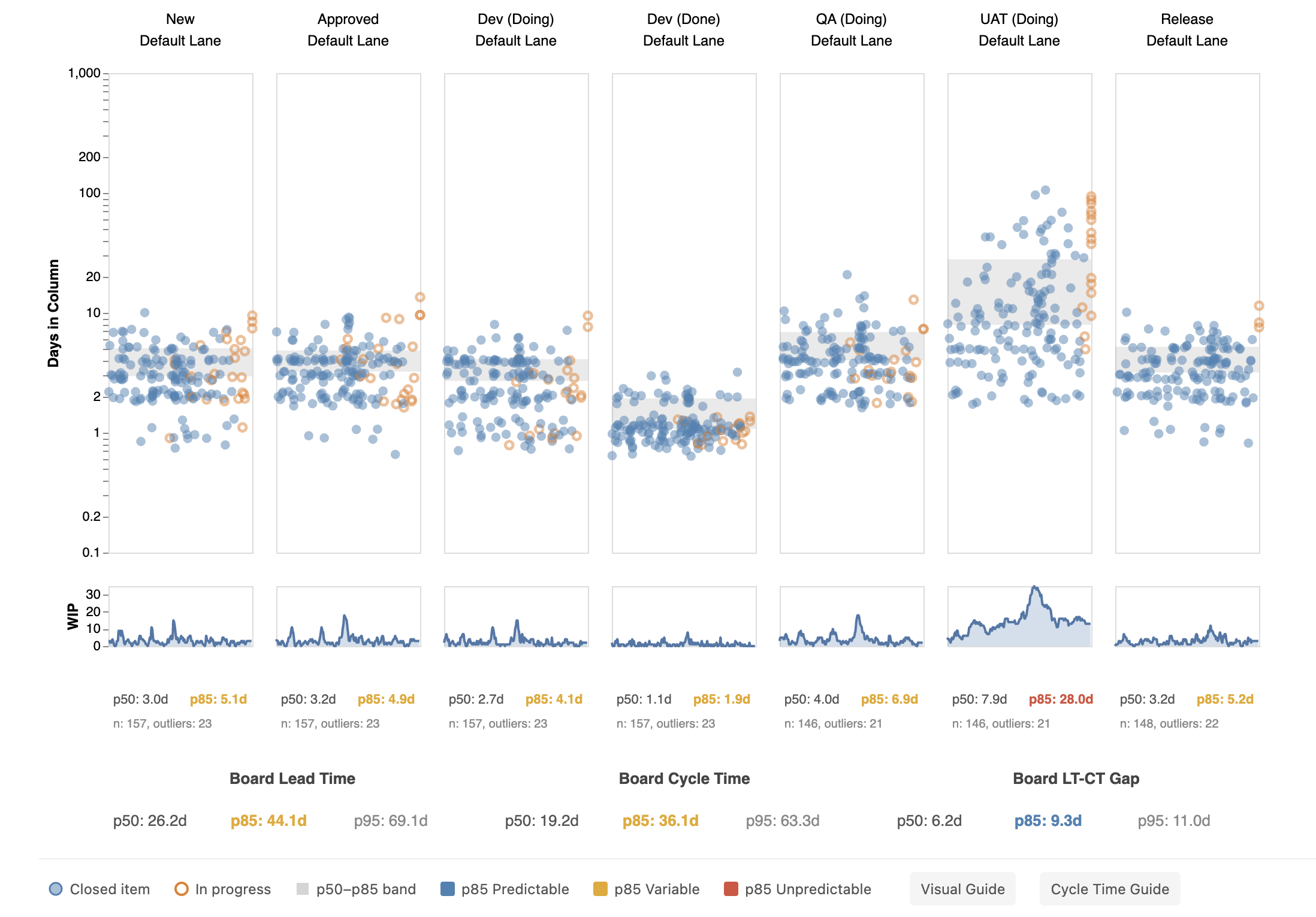
In this example, six columns have p85 values between 1.9 and 6.9 days with blue or orange variance indicators. The UAT column has a p85 of 28.0 days — red, and more than 4 times higher than any other column.
The board-level cycle time p85 jumps to 35 days even though most columns are fast and predictable. One unpredictable column dominates the board-level statistics and makes overall delivery time unreliable.
Measuring Predictability: The Variance Ratio
A useful way to quantify how predictable a column (or your whole board) is: divide p85 by p50. This ratio tells you how much spread exists between a typical item and a slow one.
| Ratio | What it means | Indicator |
|---|---|---|
| Below 1.5 | Tight and predictable | Blue |
| 1.5 to 2.0 | Moderate spread, worth watching | Orange |
| Above 2.0 | Wide spread, forecasts unreliable | Red |
A healthy column might have p50: 3 days, p85: 5 days — a ratio of 1.7. A bottleneck column might have p50: 8 days, p85: 26 days — a ratio of 3.3. The colors in the stats strip reflect this ratio directly.
To track improvement over time, compare this ratio across successive time periods. As your team addresses the root causes of a bottleneck (reducing WIP, clearing blockers faster, breaking up large items), the ratio should shrink. The dots tighten, the band narrows, the color shifts from red to orange to blue — and your forecasts get more accurate as a result.
Hover over the stats strip (column level or board level) to see the variance ratio in the tooltip.
When the Board Is Blue but Columns Aren’t
The previous section showed how one red column can drag board-level stats down. The reverse is also common and easier to miss: a board with a blue (predictable) variance ratio at the board level, while individual columns show orange or red.
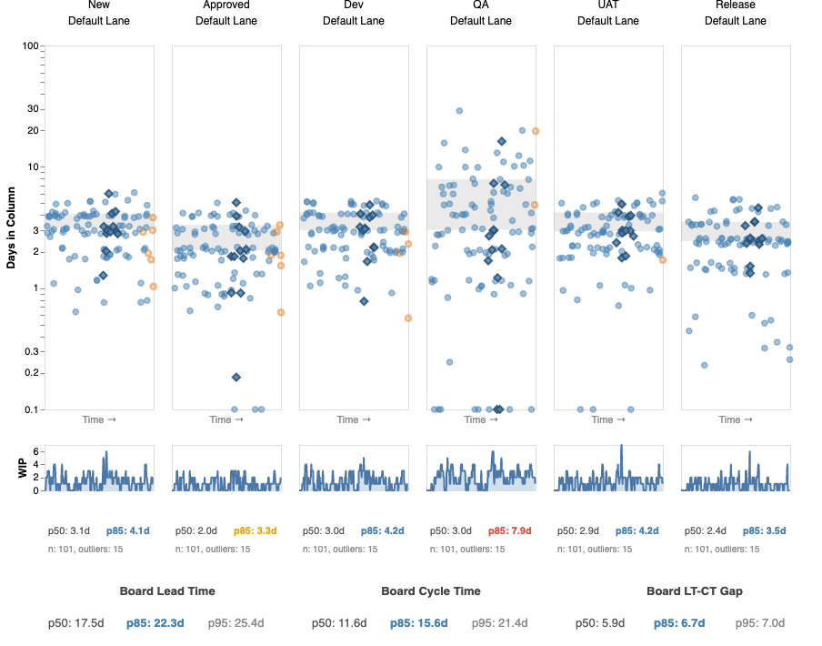
This happens because the law of large numbers smooths out column-level variance when enough items flow through. It also depends on how disruptive the problem column is relative to the rest of the board — a column with a red variance ratio but low WIP may not move the board-level needle, while a column with moderate variance but consistently high WIP can. Most items pass through the slow column quickly — it’s only some that get stuck. At the board level, those outliers blend into a distribution that still looks tight.
The board-level blue tells you that batch-level estimates are trustworthy. If you commit to delivering a cohort of 10 features, your overall timeline is reliable. But it does not mean every item’s path will be smooth. An individual item sitting in a red column right now has wide confidence intervals regardless of what the board-level stats say.
Read the two levels together:
- Board blue, columns blue — the system is predictable at every level. Forecasts are reliable for both batches and individual items.
- Board blue, some columns orange or red — batch forecasts are reliable, but individual items can get stuck in specific columns. Focus improvement on the red columns — they’re where surprises hide. The board-level number won’t improve much further until those columns tighten up.
- Board orange or red — the system is unpredictable overall. Address column-level variance first, starting with the worst offender.
Outliers: Your Best Retrospective Material
Items that land above the p85 line in a column are outliers — they took longer than 85% of completed work in that column. The stats strip shows how many outliers exist per column.
Outliers are not just statistical noise — they’re specific work items with specific stories. Right-click any column header and choose “Copy outliers” to export them to your clipboard — by column, by swim lane, or for the entire board. You can also hover individual dots above the p85 line to identify them by name. Ask: Why did this item take so long in this column? Was it blocked? Oversized? Waiting on someone?
If the same items appear as outliers across multiple columns, they likely share a structural characteristic — unclear requirements, external dependencies, or unusual complexity. Bring these specific items to your retrospective as concrete examples. A team discussing “why did item #342 take 27 days in QA” will reach more actionable conclusions than a team discussing “why is our QA p85 high.”
Forecasting Remaining Time
When a hollow dot catches your attention — especially one sitting above the p85 line — the natural next question is: how much longer?
Hover over any hollow dot to see a forecast in the tooltip:
- Remaining (p50) — half of similar items finish within this many more days
- Remaining (p85) — 85% of similar items finish within this many more days
The forecast takes into account two things: how much time the item has already spent in its current column, and how long items typically spend in each column still to come.
Current column: Rather than assuming the item will take the average amount of time, the forecast looks only at completed items that also spent at least this long in this column — and asks how much longer those items went on to take. An item that has already been in Code Review for 8 days is not like a typical item entering Code Review; it’s more like items that also stalled at 8 days.
Downstream columns: For each column the item still has to pass through, the forecast draws from the full history of completed items in that column.
Both are combined to give a single remaining time estimate — not a point prediction, but a range you can reason about.
If you see ⚠ outlier, the item has already been in its current column longer than almost all historical items — there isn’t enough data to estimate how much longer it will stay in that column. If there are columns still to come, the forecast shows a downstream-only estimate: ⚠ outlier · 2.1 d. If this is the last column before Done, both rows simply show ⚠ outlier. Either way, the warning itself is the signal — this item has already exceeded its normal range for this column.
This is most useful in dependency conversations. When a big board is full of in-progress work and someone asks “when will the thing blocking us be done?”, hovering over that item gives an honest, data-driven answer based on your team’s actual history — not a guess.
How Bottlenecks Undermine Forecasts
An unreliable column doesn’t just slow items down — it makes predictions untrustworthy for any item that hasn’t passed through it yet.
Consider two items from the same team, both flowing through a board where a single column has high variance:
Item A got through the bottleneck column quickly and reached Release. At that point, the forecast said p50: 2 days remaining, p85: 4 days. It closed 3 days later — the forecast was spot on.
Item B got stuck in the bottleneck column for 27 days. The forecast at that point said p50: 22 days remaining, p85: 38 days. It actually closed 4 days later — the forecast was wildly off.
Both forecasts were mathematically correct given the data: historical items that spent 27+ days in that column usually went on to spend much longer. Item B beat the odds, but nobody could have predicted that from the data alone. The variance itself is the problem. Until that column becomes predictable, forecasts for any item approaching it carry a wide uncertainty range.
This is why spotting bottlenecks matters beyond just throughput — it directly determines how much you can trust the forecast for any item still in flight.
Flow Efficiency: How Much Time Is Active Work
Not all time in a workflow is productive. Work often sits waiting — for a reviewer, for a dependency, for a decision — before anyone actively works on it.
Flow efficiency is the ratio of time actively worked to total lead time. A flow efficiency of 30% means that for every 10 days an item spends in your workflow, only 3 of those days involve active work. The rest is waiting.
Most teams are surprised to find their flow efficiency is lower than expected — often between 10% and 40%. This isn’t a criticism; it reflects the reality that hand-offs, queues, and dependencies are part of most workflows. But knowing your flow efficiency tells you where improvement effort will have the most impact.

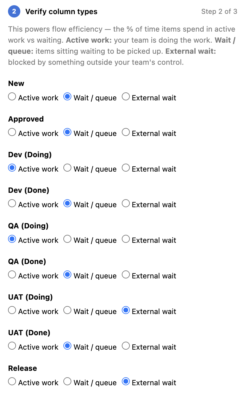
To calculate true flow efficiency in AgileViz, the AI analysis asks you to classify each column as a work column (active work happens here) or a wait column (items sit here until someone picks them up). This is covered in the Getting the Most from the AI Analysis section below.
The AI Analysis: What It Does
The Analyze tab in the sidebar sends your board’s flow stats to an AI model, which generates a structured report with observations, interpretations, and recommendations.
What the AI sees:
- Cycle time statistics (p50, p85, p95) per column
- Weekly time series — throughput and WIP per column, week over week
- Board lead time and cycle time
- Flow efficiency (if you classify your columns)
- The backlog level you selected (team vs. portfolio)
- Optional context you provide (team size, free text)
- Team name and board column names (so the report can reference your specific columns)
What the AI does not see:
- The names or content of your work items
- Sprint names, iteration paths, or area paths
- Your team’s history, structure, or commitments
- Anything outside the statistical summary of your board data
The AI report is structured in four sections:
- Situation — what the data shows
- Interpretation — a numbered list of patterns and their implications, easy to reference in group discussion
- Recommendations — prioritized actions tied to specific evidence
- Questions for Your Retrospective — discussion prompts grounded in your data
Treat the recommendations as starting points for a conversation, not directives. The AI doesn’t know your team’s context — you do.
Getting the Most from the AI Analysis
A few things significantly improve the quality of the analysis:
Classify your columns. The Analyze tab asks you to mark each column as a work column, wait column, or external wait column. This unlocks true flow efficiency calculation, which makes the analysis more precise. AgileViz pre-fills these based on column names — review them and adjust if needed. If you need to merge or hide columns first, use the Edit Visual tab; the classification list here reflects those changes.
Select at least 30 days of data. When your date range covers 30 or more days, the analysis includes weekly trend data — throughput over time, WIP changes per column, and week-over-week stability. This is what powers the temporal insights in the report (rising/falling WIP, throughput spikes, trend stability). Shorter ranges still produce useful analysis, but without the trend layer.
Set a meaningful SLA target. When asked for a target cycle time, think about what your stakeholders actually expect. If most requests are for features that should be done within two weeks, enter 14 days. The AI will assess how your current delivery rate compares.
Use the optional context field. A sentence or two about your team, the type of work, or any known constraints (a major dependency, a recent reorganization) gives the AI useful grounding for its recommendations.
Read the Questions section. The AI ends each report with questions for discussion. These are often the most valuable part — they surface the conversations that the data suggests are worth having.